Review Article
Heat transfer investigation of Non-Newtonian Fluid between two vertically infinite flat plates by numerical and analytical solutions

Pourmehran O1*, Rahimi-Gorji M2, Tavana M3, Gorji-Bandpy M4 and Ganji DD4
1Young Elites’ Sponsor Institution, Tehran, Iran
2Technical and Vocational University of Iran, Behshahr, Mazandaran, Iran
3Iran University of Science and Technology, Department of Mechanical Engineering, Tehran, Iran
4Babol Noshirvani University of Technology, Department of Mechanical Engineering, Iran
*Address for Correspondence: Dr. Pourmehran O, Young Elites’ Sponsor Institution, Tehran, Iran, Email: [email protected]
Dates: Submitted: 14 April 2017; Approved: 15 May 2017; Published: 18 May 2017
How to cite this article: Pourmehran O, Rahimi-Gorji M, Tavana M, Gorji-Bandpy M, Ganji DD. Heat transfer investigation of Non-Newtonian Fluid between two vertically infinite flat plates by numerical and analytical solutions. Ann Biomed Sci Eng. 2017; 1: 001-011. DOI: 10.29328/journal.abse.1001001
Copyright License: © 2017 Pourmehran O, et al. This is an open access article distributed under the Creative Commons Attribution License, which permits unrestricted use, distribution, and reproduction in any medium, provided the original work is properly cited.
Keywords: Natural convection; Non-Newtonian fluid; Partial differential equation; Collocation Method (CM); Numerical Method (NUM)

ABSTRACT
In natural convection, the fluid motion occurs by natural means such as buoyancy. Heat transfer by natural convection happens in many physical problems and engineering applications such as geothermal systems, heat exchangers, petroleum reservoirs and nuclear waste repositories. These problems and phenomena are modeled by ordinary or partial differential equations. In most cases, experimental solutions cannot be applied to these problems, so these equations should be solved using special techniques. In this paper, natural convection of a non-Newtonian fluid flow between two vertical flat plates is investigated analytically and numerically. Collocation Method (CM) and fourth-order Runge -Kutta numerical method (NUM) are used to solve the present problem. These methods are powerful and convenient algorithms in finding the solutions for the equations. While these are capable of reducing the size of calculations. In order to compare with exact solution, velocity and temperature profiles are shown graphically. The obtained results are valid with significant accuracy.
INTRODUCTION
Natural convection is a very important mechanism that is operative in a variety of environments from cooling electronic circuit boards in computers to causing large scale circulation in the atmosphere as well as in lakes and oceans that influences the weather. It is caused by the action of density gradients in conjunction with a gravitational field. Natural convection has attracted a great deal of attention from researchers because of its presence both in nature and engineering applications In nature, convection cells formed from air rising above sunlight-warmed land or water are a major feature of all weather systems. In engineering applications, convection is commonly visualized in the formation of micro-structures during the cooling of molten metals, and fluid flows around shrouded heat-dissipation fins, and solar ponds. A very common industrial application of natural convection is free air cooling without the aid of fans: this can happen on small scales (computer chips) to large scale process equipment. Also heat transfer by natural convection occurs in many physical problems and engineering applications such as geothermal systems, heat exchangers, chemical catalytic reactors, fiber and granular insulation, packed beds, petroleum reservoirs and nuclear waste repositories. In review of its importance, the flow of Newtonian and non-Newtonian fluids through two infinite parallel vertical plates has been investigated by numerous authors. In this system heat is transferred from a vertical plate to a fluid moving parallel to it by natural convection.
This will occur in any system wherein the density of the moving fluid varies with position. These phenomena will only be of significance when the moving fluid is minimally affected by forced convection [1]. The natural convection problem between vertical flat plates for a certain class of non-Newtonian fluids has been carried out by Bruce and Na [2]. Also other laminar natural convection problems involving heat transfer have been studied in [3]. However, Rajagopal presented a complete thermodynamic analysis of the constitutive functions [4]. These scientific problems and phenomena are modeled by ordinary or partial differential equations. In recent years, much attention has been devoted to the newly developed methods to construct an analytic solution of these equations; such as the perturbation method [5], variational techniques [6], Collocation Method (CM) and fourth-order Runge -Kutta numerical method (NUM) [7-15]. These methods have been used by some authors in wide variety of scientific and engineering applications to solve different types of governing differential equations: linear and nonlinear, homogeneous and non-homogeneous, and coupled and decoupled as well. Several researchers studied various problems by this accurate method [16-22]. These methods offer highly accurate successive approximations of the solution. Etbaeitabari and Domairy have studied analytically with Reconstruction of Variational Iteration Method (RVIM) scheme on present problem and their results had very good agreement with the older researches [23]. Therefore, Collocation Method was used to find efficient, reliable and precise polynomial solutions. Thus in this work we examine the natural convection of a non-Newtonian fluid, namely the Rivlin -Ericksen fluid of grade three, between two infinite parallel vertical flat plates to obtain its solution using CM and NUM.
Description of the problem
A schematic of the problem is shown in figure 1. It consists of two flat plates that can be positioned vertically. A non-Newtonian fluid is in two flat plates a distance 2b apart. The walls at x=+b and x=−b are held at constant temperatures φ2 and φ1 respectively, where φ1>φ2 . This difference in temperature causes the fluid near the wall at x=−b to rise and the fluid near the wall at x=+b to fall. Rajagopal [4] has demonstrated that by using the similarity variables:
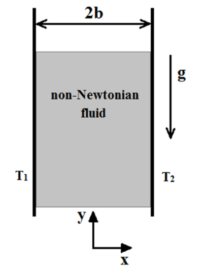
Figure 1: Schematic diagram of the problem under consideration.
The Navier-Stokes and Energy equations can be reduced to the following pair of ordinary differential equations [5]:
Where c is the specific heat of the fluid. The appropriate boundary conditions are:
After that, we solve the system of Eqs. (2) and (3) by using the CM and NUM. The equations are coupled and highly non-linear.
MATHEMATICAL METHODS
Before presenting the results, it is necessary to provide some background knowledge about the mathematical methods employed. Therefore, in this section, some basic relationships and theories concerning Collocation method (CM) and fourth order Runge-Kutta Numerical Method are presented.
There are some simple and accurate approximation techniques for solving differential equations called the Weighted Residuals Methods (WRMs). Collocation (CM), Galerkin (GM) and Least Square (LSM) are examples of the WRMs. Collocation Method (CM) were firstly introduced by Ozisik [24] for solving differential equations in heat transfer problems. Stern and Rasmussen [25] used collocation method for solving a third order linear differential equation. Vaferi et al. [26] studied the feasibility of applying of Orthogonal Collocation method to solve diffusivity equation in the radial transient flow system.
Many advantages of CM compared to other analytical make it more valuable and motivate researchers to use it for solving problems. Some of these advantages are listed below [14].
a) WRMs solve the equations directly and no simplifications are needed.
b) They do not need any perturbation, linearization or small parameter versus Homotopy Perturbation Method (HPM) and Parameter Perturbation Method (PPM).
c) They are simple and powerful compared to numerical methods and achieve final results faster than numerical procedures while their results are acceptable and have excellent agreement with numerical outcomes, furthermore their accuracy can be increased by increasing the statements of the trial functions.
d) They don’t need to determine the auxiliary parameter and auxiliary function versus Homotopy Analysis Method (HAM).
Collocation Method (CM)
For conception of the main idea of this method, suppose a differential operator D is acted on a function V to produce a function p:
We wish to approximate V by a function ṽ, which is a linear combination of basic functions chosen from a linearly independent set. That is,
Now, when substituted into the differential operator, D, the result of the operations is not p(X). Hence an error or residual will exist:
The notion in the Collocation is to force the residual to zero in some average sense over the domain. That is,
where the number of weight functions Wi is exactly equal the number of unknown constants in ṽ. The result is a set of n algebraic equations for the unknown constants .The value of n has been guessed. For collocation method, the weighting functions are taken from the family of Dirac functions in the domain. That is Wi(Xi) = (X-Xi). The Dirac function has the property of
And residual function in Eq. (9) must be forced to be zero at specific points.
Fourth order Runge-Kutta Method (NUM)
It is obvious that the type of the current problem is boundary value problem (BVP) and the appropriate method needs to be chosen. The available sub-methods in the Maple 17.0 are a combination of the base schemes; trapezoid or midpoint method. There are two major considerations when choosing a method for a problem. The trapezoid method is generally efficient for typical problems, but the midpoint method is so capable of handling harmless end-point singularities that the trapezoid method cannot. The midpoint method, also known as the fourth-order Runge-Kutta-Fehlberg method, improves the Euler method by adding a midpoint in the step which increases the accuracy by one order. Thus, the midpoint method is used as a suitable numerical technique in present study [9].
RESULTS AND DISCUSSION
The applicability of the presented methods for the nonlinear equation of natural convection will be illustrated in the following section. In order to measure the accuracy of the results, NUM has been used here for the derived non-linear ODE, given in Eqs.(2),(3). A Maple code was used to find the numerical solution of the present boundary value problem (BVP).
Approximate solution with CM
In present study, the fluid is considered non-Newtonian fluid and governing equations for investigation of temperature and velocity profiles of natural convection of non-Newtonian fluid between two parallel plates are solved by CM and NUM. For solving Eqs. (2) and (3) by WRMs, because trial function must satisfy the boundary condition in Eq. (5), so each statement in φ(ξ) and U(ξ) should contain t to satisfy boundary condition in ξ=+1 and ξ=-1. In this study, one statement is considered for velocity profile and one statement is considered for temperature profile and as explained in above WRMs advantages, accuracy of results can be increased by increasing the number of statements. Which satisfy the boundary condition in Eq. (5) and by setting it into Eqs. (2) and (3), residual functions, Ri(c,ξ), will be found. On the other hand, the residual functions must be close to zero.
In this work, approximate polynomials for φ(ξ) and U(ξ) are as follows:
For example, U(ξ) and φ(ξ) by using Collocation Method with Pr=δ=E=1 are as follows:
The results of the different methods of CM and NUM are compared in figures 2 and 3. Figures 2 shows the non-dimensional temperature φ(ξ), while figures 3 shows the comparison of the non-dimensional velocity U(ξ) of CM and the numerical method (NUM) for known values of the parameters E=1 and Pr=1. Figures 4 and 5 illustrate effect of δ on the non-dimensional temperature φ(ξ) and velocity U(ξ) as well. Figure 5 Indicates that by increasing δ the amount of temperature increases for positive region and the same treatment is obvious for the minus region. And also as it is obvious in figures 4, the velocity for positive values of x increases by increasing δ. But there is an opposite manner in the minus region. Figures 6 and 7 show the result of φ(ξ) and U(ξ) for various Prandtl number Pr when δ=1 and E=1. According to figures 6 and 7 by increasing Pr, the non-dimensional velocity U(ξ) and temperature φ(ξ) increased. Also the same result is indicated increasing E, in figures 8 and 9. According to tables 1 and 2 these approximate analytical solutions are in excellent agreement with the corresponding numerical solutions. In these tables different iterations of CM are tabulated to show the power of this method in finding an accurate approximation. It is obvious in tables 3 and 4 that show the errors.
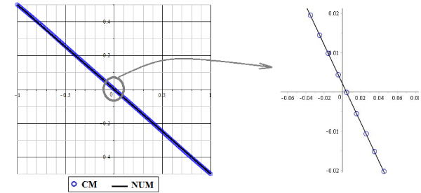
Figure 2: The result of φ(ξ) for Pr=1 and E=1 compared to the numerical method.
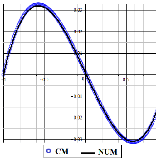
Figure 3: The result of U(ξ) for δ=0.1, Pr=1, and E=1 compared to the numerical method.
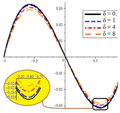
Figure 4: The result of U(ξ) for various δ when Pr=1 and E=1.
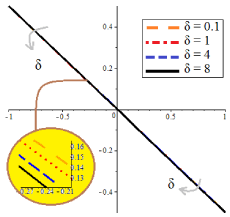
Figure 5: The result of φ (ξ) for various δ when Pr =1 and E=1.
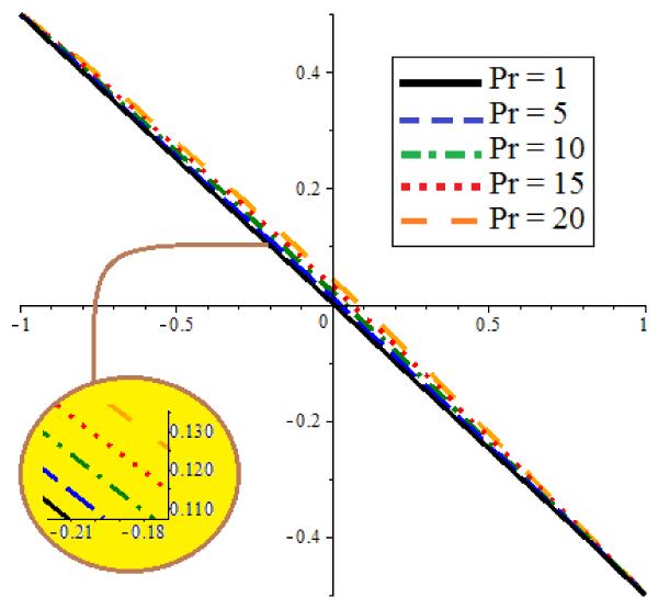
Figure 6: The result of φ(ξ) for various Pr when δ=1 and E=1.
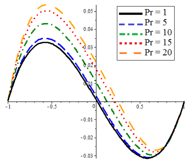
Figure 7: The result of U(ξ) for various Pr when δ=1 and E=1.
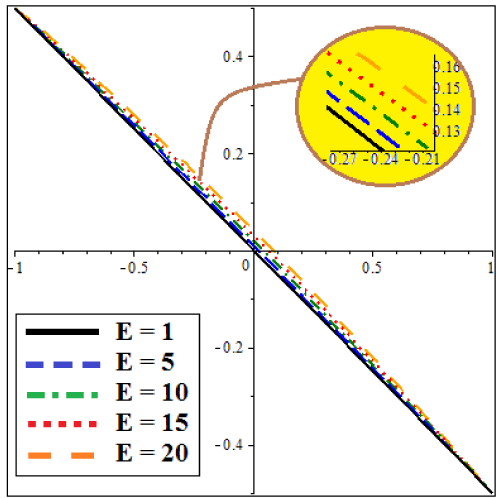
Figure 8: The result of φ(ξ) for various E when δ=1 and Pr=1.
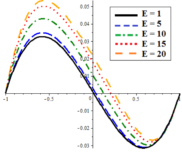
Figure 9: The result of U(ξ) for various E when δ=1 and Pr=1
| Table 1: The results of CM and NM methods for U(ξ) and φ(ξ) when δ = 4, Pr = 1, and E = 1. | |||||
| Pr = 1; E = 1; δ = 4 | |||||
| ξ | θ | U | |||
| CM | NUM | CM | NUM | ||
| -1 | 0.500000000 | 0.500000000 | 0.000000000 | 0.000000000 | |
| -0.9 | 0.452516012 | 0.450418067 | 0.013645139 | 0.012810381 | |
| -0.8 | 0.404091293 | 0.400697970 | 0.023439046 | 0.022152888 | |
| -0.7 | 0.354556328 | 0.350915046 | 0.029377443 | 0.027990642 | |
| -0.6 | 0.304163611 | 0.301112709 | 0.031769304 | 0.030475055 | |
| -0.5 | 0.253330569 | 0.251307960 | 0.031096811 | 0.029966609 | |
| -0.4 | 0.202464206 | 0.201498915 | 0.027915659 | 0.026968718 | |
| -0.3 | 0.151855818 | 0.151672875 | 0.022789957 | 0.022030455 | |
| -0.2 | 0.101634078 | 0.101813287 | 0.016255955 | 0.015682722 | |
| -0.1 | 0.051764822 | 0.051904905 | 0.008808826 | 0.008417987 | |
| 0 | 0.002085872 | 0.001937189 | 0.000906756 | 0.000695388 | |
| 0.1 | -0.047634795 | -0.048093776 | -0.007013448 | -0.007044126 | |
| 0.2 | -0.097629204 | -0.098184628 | -0.014514982 | -0.014359761 | |
| 0.3 | -0.148059532 | -0.148325269 | -0.021139661 | -0.020792750 | |
| 0.4 | -0.198959941 | -0.198500679 | -0.026392308 | -0.025850830 | |
| 0.5 | -0.250201761 | -0.248694210 | -0.029736676 | -0.029002085 | |
| 0.6 | -0.301493695 | -0.298892655 | -0.030608656 | -0.029693151 | |
| 0.7 | -0.352428738 | -0.349093159 | -0.028452551 | -0.027410767 | |
| 0.8 | -0.402589465 | -0.399311352 | -0.022786181 | -0.021779659 | |
| 0.9 | -0.451723381 | -0.449589051 | -0.013300571 | -0.012633745 | |
| 1 | -0.500000000 | -0.500000000 | 0.000000000 | 0.000000000 | |
| Table 2: The results of CM and NM methods for U(ξ) and φ(ξ) when δ=1, Pr=1, and E=1. Pr=1; E=1; δ=1 |
|||||
| ξ | θ | U | |||
| CM | NUM | CM | NUM | ||
| -1 | 0.500000000 | 0.500000000 | 0.000000000 | 0.000000000 | |
| -0.9 | 0.452569915 | 0.450437787 | 0.014313266 | 0.013879168 | |
| -0.8 | 0.404179726 | 0.400729470 | 0.024301242 | 0.023609233 | |
| -0.7 | 0.354655676 | 0.350957352 | 0.030256206 | 0.029479743 | |
| -0.6 | 0.304255411 | 0.301166316 | 0.032617829 | 0.031881091 | |
| -0.5 | 0.253405244 | 0.251373033 | 0.031903702 | 0.031275100 | |
| -0.4 | 0.202520937 | 0.201575073 | 0.028660284 | 0.028161936 | |
| -0.3 | 0.151900082 | 0.151759124 | 0.023431349 | 0.023053645 | |
| -0.2 | 0.101674141 | 0.101907811 | 0.016741027 | 0.016458246 | |
| -0.1 | 0.051808216 | 0.052004951 | 0.009088500 | 0.008873410 | |
| 0 | 0.002136615 | 0.002039244 | 0.000951458 | 0.000786884 | |
| 0.1 | -0.047577719 | -0.047993544 | -0.007204613 | -0.007319218 | |
| 0.2 | -0.097571841 | -0.098089805 | -0.014914227 | -0.014962388 | |
| 0.3 | -0.148011443 | -0.148238730 | -0.021699695 | -0.021653706 | |
| 0.4 | -0.198931424 | -0.198424377 | -0.027061833 | -0.026893477 | |
| 0.5 | -0.250200322 | -0.248629252 | -0.030476515 | -0.030170673 | |
| 0.6 | -0.301520544 | -0.298839494 | -0.031399963 | -0.030969026 | |
| 0.7 | -0.352476329 | -0.349051651 | -0.029285719 | -0.028782626 | |
| 0.8 | -0.402641363 | -0.399280914 | -0.023616192 | 0.023142149 | |
| 0.9 | -0.451758001 | -0.449570295 | -0.013951711 | -0.013647987 | |
| 1 | -0.500000000 | -0.500000000 | 0.000000000 | 0.000000000 | |
| Table 3: Error for U(ξ) and φ(ξ) when δ=4, Pr=1, and E=1. Pr=1; E=1; δ= 4 | ||
| ξ | U | θ |
| Error % | Error % | |
| -1 | 0.000000 | 0.000000 |
| -0.9 | 3.127690 | 0.473346 |
| -0.8 | 2.931094 | 0.860994 |
| -0.7 | 2.633888 | 1.053781 |
| -0.6 | 2.310895 | 1.025710 |
| -0.5 | 2.009911 | 0.808444 |
| -0.4 | 1.769578 | 0.469236 |
| -0.3 | 1.638372 | 0.092883 |
| -0.2 | 1.718174 | 0.229295 |
| -0.1 | 2.423984 | 0.378301 |
| 0 | 20.91470 | 4.774859 |
| 0.1 | 1.565808 | 0.866419 |
| 0.2 | 0.321878 | 0.528051 |
| 0.3 | 0.212383 | 0.153325 |
| 0.4 | 0.626012 | 0.255537 |
| 0.5 | 1.013704 | 0.631892 |
| 0.6 | 1.391508 | 0.897154 |
| 0.7 | 1.747903 | 0.981138 |
| 0.8 | 2.020484 | 0.841625 |
| 0.9 | 2.225413 | 0.486621 |
| 1 | 0.000000 | 0.000000 |
| Table 4: Error for U(ξ) and φ(ξ) when δ=1, Pr=1, and E=1. Pr=1; E=1; δ=1 |
||
| ξ | U | θ |
| Error % | Error % | |
| -1 | 0.000000 | 0.000000 |
| -0.9 | 6.516258 | 0.465777 |
| -0.8 | 5.805824 | 0.846853 |
| -0.7 | 4.954514 | 1.037653 |
| -0.6 | 4.246914 | 1.013209 |
| -0.5 | 3.771540 | 0.804833 |
| -0.4 | 3.511259 | 0.479055 |
| -0.3 | 3.447510 | 0.120617 |
| -0.2 | 3.655183 | 0.176018 |
| -0.1 | 4.642907 | 0.269885 |
| 0 | 3.395740 | 7.675189 |
| 0.1 | 0.435506 | 0.954346 |
| 0.2 | 1.080946 | 0.565693 |
| 0.3 | 1.668421 | 0.179158 |
| 0.4 | 2.094628 | 0.231366 |
| 0.5 | 2.532893 | 0.606186 |
| 0.6 | 3.083219 | 0.870226 |
| 0.7 | 3.800640 | 0.955498 |
| 0.8 | 4.621387 | 0.820942 |
| 0.9 | 5.278140 | 0.474729 |
| 1 | 0.000000 | 0.000000 |
CONCLUSIONS
In this paper, natural convection of a non-Newtonian fluid flow between two vertical flat plates is investigated analytically and numerically. Collocation Method (CM) and fourth-order Runge-Kutta numerical method (NUM) are used to solve the present problem. The proposed method overcame on nonlinearity without using restrictive assumptions or linearization. The following main points can be concluded from the present study.
• The results of CM are in excellent agreement with numerical ones. Also this method is simple, powerful and efficient techniques for finding analytical solutions in science and engineering non-linear differential equations which reduces the size of calculations.
• The figures bring out clearly the effect of δ on the non-dimensional temperature φ(ξ) and velocity U(ξ) as well. While δ increases the amount of temperature increases at positive region and decreases at minus region of x.
• by increasing Pr the non-dimensional velocity U(ξ) and temperature φ(ξ) increased respectively and by increasing E treatment of the non-dimensional velocity U(ξ) and temperature φ(ξ) are additive.
REFERENCES
- McCabe WL, Smith JC, Harriott P. Unit operations of chemical engineering. McGraw-Hill New York. 1993. Ref.: https://goo.gl/ZPbfG3
- Bruce RW, Na TY. Natural convection flow of Powell-Eyring fluids between two vertical flat plates. ASME. 1967. Ref.: https://goo.gl/kZIHjc
- Shenoy AV, Mashelkar RA. Thermal convection in non-Newtonian fluids. Advances in heat transfer. 1982; 15: 143-225. Ref.: https://goo.gl/5CM5CD
- Dunn JE, Rajagopal KR. Fluids of differential type: critical review and thermodynamic analysis. International Journal of Engineering Science. 1995; 33: 689-729. Ref.: https://goo.gl/yOaMb0
- Nayfeh AH. Perturbation methods. 2008. Ref.: https://goo.gl/gq0nGe
- Ganji SS, Ganji DD, Karimpour S. He's energy balance and He's variational methods for nonlinear oscillations in engineering. International Journal of Modern Physics B. 2009; 23: 461-471. Ref.: https://goo.gl/SVMwsa
- Rahimi-Gorji M, Pourmehran O, Gorji-Bandpy M, Ganji D. Unsteady squeezing nanofluid simulation and investigation of its effect on important heat transfer parameters in presence of magnetic field. Journal of the Taiwan Institute of Chemical Engineers. 2016; 67: 467-475. Ref.: https://goo.gl/lO2LpS
- Pourmehran O, Gorji TB, Gorji-Bandpy M. Magnetic drug targeting through a realistic model of human tracheobronchial airways using computational fluid and particle dynamics. Biomechanics and modeling in mechanobiology. 2016; 15: 1355-1374. Ref.: https://goo.gl/0et8vE
- Pourmehran O, Rahimi-Gorji M, Ganji D. Heat transfer and flow analysis of nanofluid flow induced by a stretching sheet in the presence of an external magnetic field. Journal of the Taiwan Institute of Chemical Engineers. 2016; 65: 162-171. Ref.: https://goo.gl/Wqeh6m
- Rahimi-Gorji M, Pourmehran O, Gorji-Bandpy M, Gorji T. CFD simulation of airflow behavior and particle transport and deposition in different breathing conditions through the realistic model of human airways. Journal of Molecular Liquids. 2015; 209: 121-133. Ref.: https://goo.gl/7pVooK
- Pourmehran O, Rahimi-Gorji M, Gorji-Bandpy M, Gorji TB. Simulation of magnetic drug targeting through tracheobronchial airways in the presence of an external non-uniform magnetic field using Lagrangian magnetic particle tracking. Journal of Magnetism and Magnetic Materials. 2015; 393: 380-393. Ref.: https://goo.gl/KSc8EI
- Rahimi-Gorji M, Pourmehran O, Gorji-Bandpy M, Ganji DD. An analytical investigation on unsteady motion of vertically falling spherical particles in non-Newtonian fluid by Collocation Method. Ain Shams Engineering Journal. 2015; 6: 531-540. Ref.: https://goo.gl/ZCzxl4
- Pourmehran O, Rahimi-Gorji M, Hatami M, Sahebi SAR, Domairry G. Numerical optimization of microchannel heat sink (MCHS) performance cooled by KKL based nanofluids in saturated porous medium. Journal of the Taiwan Institute of Chemical Engineers. 2015; 55: 49-68. Ref.: https://goo.gl/uZd5CO
- Pourmehran O, Rahimi-Gorji M, Gorji-Bandpy M, Ganji D. Analytical investigation of squeezing unsteady nanofluid flow between parallel plates by LSM and CM. Alexandria Engineering Journal. 2015; 54: 17-26. Ref.: https://goo.gl/YK3gCu
- Rahimi-Gorji M, Pourmehran O, Hatami M, Ganji D. Statistical optimization of microchannel heat sink (MCHS) geometry cooled by different nanofluids using RSM analysis. The European Physical Journal Plus. 2015; 130: 22. Ref.: https://goo.gl/f5oKpj
- M Hammes, M Boghosian, K Cassel, S Watson, B Funaki, et al. Increased Inlet Blood Flow Velocity Predicts Low Wall Shear Stress in the Cephalic Arch of Patients with Brachiocephalic Fistula Access. PloS one. 2016; 11. Ref.: https://goo.gl/i3sGCg
- SM Javid Mahmoudzadeh Akherat, Kevin Cassel, Michael Boghosian, Promila Dhar, Mary Hammes. Are Non-Newtonian Effects Important in Hemodynamic Simulations of Patients With Autogenous Fistula?. Journal of Biomechanical Engineering. 2017; 139. Ref.: https://goo.gl/y9Svvn
- M Fakour, DD Ganji, A Khalili, A Bakhshi. HEAT TRANSFER IN NANOFLUID MHD FLOW IN A CHANNEL WITH PERMEABLE WALLS. Heat Transfer Research. 2017; 48. Ref.: https://goo.gl/pg9hvr
- M Fakour, A Vahabzadeh, DD Ganji. Study of heat transfer and flow of nanofluid in permeable channel in the presence of magnetic field. Propulsion and Power Research. 2015; 4: 50-62. Ref.: https://goo.gl/GXH0rG
- M Fakour, DD Ganji, M Abbasi. Scrutiny of underdeveloped nanofluid MHD flow and heat conduction in a channel with porous walls. Case Studies in Thermal Engineering. 2014; 4: 202-214. Ref.: https://goo.gl/14dEOB
- M Fakour, A Vahabzadeh, DD Ganji, M Hatami. Analytical study of micropolar fluid flow and heat transfer in a channel with permeable walls. Journal of Molecular Liquids. 2015; 204: 198-204. Ref.: https://goo.gl/k4kefw
- A Rahbari, M Fakour, A Hamzehnezhad, MA Vakilabadi, DD Ganji. Heat transfer and fluid flow of blood with nanoparticles through porous vessels in a magnetic field: A quasi-one dimensional analytical approach. Mathematical Biosciences. 2017; 283: 38-47. Ref.: https://goo.gl/81Hd29
- A Etbaeitabari, M Barakat, AA Imani, G Domairry, P Jalili. An analytical heat transfer assessment and modeling in a natural convection between two infinite vertical parallel flat plates. Journal of Molecular Liquids. 2013; 188: 252-257. Ref.: https://goo.gl/ws2q0Z
- MN Ozisik. Heat conduction. John Wiley & Sons. 1993. Ref.: https://goo.gl/PNxseq
- Ralph H Stern, Henning Rasmussen. Left ventricular ejection: model solution by collocation, an approximate analytical method. Computers in biology and medicine. 1996; 26: 255-261. Ref.: https://goo.gl/t5prSP
- B Vaferi,V Salimi, D Dehghan Baniani, A. Jahanmiri, S Khedri, Prediction of transient pressure response in the petroleum reservoirs using orthogonal collocation. Journal of Petroleum Science and Engineering, (2012) 98:156-163.Ref.: https://goo.gl/E7kEwS